The Pandora Box: Interaction

If you wish, we could go on and carry out every detail of the quantum free scalar, i.e., it is exactly solved. But that's too much for us. All the introduced devices in the previous section are enough to let us peek into the world of interacting field theories, meaning that the fields are no longer decomposed into decoupled wave modes. In our interpretation where excitation of modes are recognized as particles, this indicates interaction between them: as time elapses, modes can cease or arise in accord to each other. However, all those interpretations usually only make sense when the interactions are small, so the theory can be thought as modified upon the free theory, or equivalently, free particles. And indeed, we will only work with perturbative interactions, though another important reason for that is nobody knows how to properly deal with strongly coupled quantum fields.

Even if we are to work with perturbative calculations, the interacting theories are incredibly complicated, and we will inevitably run into the problem of infinities and renormalization. In fact, one would fairly say that the entire complication of QFT comes from interactions. In this section, we will avoid renormalization as much as possible, and focus on introducing the formalism. Even in this case, there are still many things to say.

The Interaction Picture

We all know that the Schrödinger picture involves evolving states and stationary operators, while the Heisenberg picture involves stationary states and evolving operators. The key idea of the interaction picture is that, find a way to evolve both the states and the operators, so that the time evolution looks as if only part of the Hamiltonian is relevant. We denote a Schrödinger picture state by Ψ(t)S\ket{\Psi(t)}_S. Also, we assume a Hamiltonian of the form

H=H0+HintH=H_0+H_\text{int}

Although the separation of the Hamiltonian is arbitrary, we conventionally separate it into a free part and an interaction part.

Then, we define the transformation from the Schrödinger picture to the interaction picture, with identification at t=t0t=t_0

Ψ(t)I=exp{iH0,S(tt0)}Ψ(t)SΨ(t0)I=Ψ(t0)S\ket{\Psi(t)}_I=\exp{\{iH_{0,S} (t-t_0)\}}\ket{\Psi(t)}_S\quad\ket{\Psi(t_0)}_I=\ket{\Psi(t_0)}_S

and the corresponding transformation of operators

OI(t)=exp{iH0,S(tt0)}OSexp{iH0,S(tt0)}\mathcal{O}_I(t)=\exp{\{iH_{0,S} (t-t_0)\}}\mathcal{O}_S\exp{\{-iH_{0,S} (t-t_0)\}}

With all the rules, we can now transform the Schrödinger equation

iΨ(t)Idt=id(exp{iH0,S(tt0)}Ψ(t)S)dt=exp{iH0,S(tt0)}H0,SΨ(t)S+iexp{iH0,S(tt0)}Ψ(t)Sdt=exp{iH0,S(tt0)}H0,Sexp{iH0,S(tt0)}exp{iH0,S(tt0)}Ψ(t)S+exp{iH0,S(tt0)}HSexp{iH0,S(tt0)}exp{iH0,S(tt0)}Ψ(t)S=H0,I(t)Ψ(t)I+HI(t)Ψ(t)I=Hint,I(t)Ψ(t)I\begin{aligned} i\frac{\ket{\Psi(t)}_I}{dt}&=i\frac{d\left(\exp{\{iH_{0,S} (t-t_0)\}}\ket{\Psi(t)}_S\right)}{dt}\\ &=-\exp{\{iH_{0,S} (t-t_0)\}}H_{0,S}\ket{\Psi(t)}_S+i\exp{\{iH_{0,S} (t-t_0)\}}\frac{\ket{\Psi(t)}_S}{dt}\\ &=-\exp{\{iH_{0,S} (t-t_0)\}}H_{0,S}\exp{\{-iH_{0,S} (t-t_0)\}}\exp{\{iH_{0,S} (t-t_0)\}}\ket{\Psi(t)}_S\\ &\quad+\exp{\{iH_{0,S} (t-t_0)\}}H_S\exp{\{-iH_{0,S} (t-t_0)\}}\exp{\{iH_{0,S} (t-t_0)\}}\ket{\Psi(t)}_S\\ &=-H_{0,I}(t)\ket{\Psi(t)}_I+H_{I}(t)\ket{\Psi(t)}_I\\ &=H_{\text{int},I}(t)\ket{\Psi(t)}_I \end{aligned}

Although not that important, we can directly read off the evolution of the operator from the definition of transformation

idOI(t)dt=[OI(t),H0,I(t)]i\frac{d\mathcal{O}_I(t)}{dt}=\comm{\mathcal{O}_I(t)}{H_{0,I}(t)}

much like the Heisenberg picture.

The transformed Schrödinger equation can be solved iteratively by

Ψ(t)I=(1+it0tHint,I(τ)dτ+i2t0tt0τHint,I(τ)Hint,I(τ)dτdτ+)Ψ(t0)I=(1+it0tHint,I(τ)dτ+i22!t0tt0tT[Hint,I(τ)Hint,I(τ)]dτdτ+)Ψ(t0)I=T[exp{it0tHint,I(τ)dτ}]Ψ(t0)I\begin{aligned} \ket{\Psi(t)}_I&=\left(1+i\int_{t_0}^t H_{\text{int},I}(\tau)d\tau+i^2\int_{t_0}^t\int_{t_0}^\tau H_{\text{int},I}(\tau)H_{\text{int},I}(\tau^\prime)d\tau^\prime d\tau+\cdots\right)\ket{\Psi(t_0)}_I\\ &=\left(1+i\int_{t_0}^t H_{\text{int},I}(\tau)d\tau+\frac{i^2}{2!}\int_{t_0}^t\int_{t_0}^t T\left[H_{\text{int},I}(\tau)H_{\text{int},I}(\tau^\prime)\right]d\tau^\prime d\tau+\cdots\right)\ket{\Psi(t_0)}_I\\ &=T\left[\exp{\left\{i\int_{t_0}^t H_{\text{int},I}(\tau) d\tau\right\}}\right]\ket{\Psi(t_0)}_I \end{aligned}

The first line can be checked to solve the equation by direct differentiation, and in the second line we inserted the time ordering to unify the interval of integral, with a 1n!\frac{1}{n!} accounting for the multiplicity. The third line is a compact way to denote this.

This is the celebrated Dyson series, the explicit evolution of states in the interaction picture, which is also significant in time dependent perturbation. It is worth pointing out that so far every results are exact and non-perturbative, but this scheme is especially suitable for perturbation because if HintH_\text{int} is controlled by some small parameter ϵ\epsilon, then the Dyson series make explicit the contributions of different orders of ϵ\epsilon into the time evolution, and one can reasonably cutoff at some finite order of ϵ\epsilon to get perturbative results.

Physical Vacuum

It is time to utilise the device to the real scalar theory. Let us introduce an interaction to the Klein-Gordon field by modifying the Lagrangian density as

L=12μϕμϕ12m2ϕ2λ4!ϕ4\mathcal{L}=\frac12\partial^\mu\phi\partial_\mu\phi-\frac12 m^2\phi^2-\frac{\lambda}{4!}\phi^4

so that the corresponding Hint\mathbf{H}_\text{int} is

Hint=d3xλ4!ϕ4\mathbf{H}_\text{int}=\int d^3x\,\frac{\lambda}{4!}\phi^4

Here we begin to enjoy the first elegance provided by the interaction picture: since the operators are just evolved with the free part, the time-dependent ϕ(x)\phi(x) we worked out is still available, just with the creation and annihilation operators in it replaced with the corresponding interaction picture one. For this is the general case, we will drop the subscripts indicating pictures without ambiguity.

But we also run into our first problem: what is the vacuum now? Note that we have two “vacua", one that is annihilated by the annihilation operator ap0=0\annhil{a}{p}\ket{0}=0, and another that is the lowest-energy eigenstate of the full Hamiltonian. In free theories, the two coincides. But since we modified the Hamiltonian, we can no longer expect that1, and the de facto vacuum we should look for is, of course, the latter one, which we will call it the physical vacuum2. However, the creation annihilation description is too good to dispose, and it is pleasing if we can find the relation between the two.

For convenience, we will denote the evolution operator by

U(t,t0)T[exp{it0tHint(τ)dτ}]U(t,t_0)\equiv T\left[\exp{\left\{i\int_{t_0}^t \mathbf{H}_{\text{int}}(\tau) d\tau\right\}}\right]

and the energy eigenstate of the full Hamiltonian by Ω\ket{\Omega} and nn1\ket{n}\,n\geq1. Then if we evolve the free vacuum 0\ket{0}

U(t,t0)0=Ω|0eiE0(tt0)Ω+n=1n|0eiEn(tt0)nU(t,t_0)\ket{0}=\braket{\Omega}{0}e^{-iE_0(t-t_0)}\ket{\Omega}+\sum_{n=1}^\infty \braket{n}{0}e^{-iE_n(t-t_0)}\ket{n}

It is satisfying if states with higher energy would die out. In principle, we can imagine a process where the interaction is turned off (i.e. λ=0\lambda=0) at some distant past, and then adiabatically turned on, so that the ground state evlolved to the ground state. We can implement this without being rigorous by pushing t0t_0 to the far past while it takes on a small imaginary part (characterizing the dissipation caused by the adiabatic process).

limT(1iϵ)U(t,T)0=Ω|0eiE0(t+T)Ω\lim_{T\to (1-i\epsilon)\infty}U(t,-T)\ket{0}=\braket{\Omega}{0}e^{-iE_0(t+T)}\ket{\Omega}

We can repeat the process for Ω\bra{\Omega}

0U(t,t0)=Ω0|ΩeiE0(tt0)+n=1n0|neiEn(tt0)\bra{0}U(t,t_0)^\dagger=\bra{\Omega}\braket{0}{\Omega}e^{iE_0(t-t_0)}+\sum_{n=1}^\infty \bra{n}\braket{0}{n}e^{iE_n(t-t_0)} limT(1iϵ)0U(T,t)=Ω0|ΩeiE0(Tt)\lim_{T\to (1-i\epsilon)\infty}\bra{0}U(T,t)=\bra{\Omega}\braket{0}{\Omega}e^{-iE_0(T-t)}

Therefore, we have isolated the physical vacuum

{Ω=limT(1iϵ)(Ω|0eiE0(t+T))1U(t,T)0Ω=limT(1iϵ)(0|ΩeiE0(Tt))10U(T,t)\begin{cases} \ket{\Omega}=\lim_{T\to (1-i\epsilon)\infty}(\braket{\Omega}{0}e^{-iE_0(t+T)})^{-1}U(t,-T)\ket{0}\\ \bra{\Omega}=\lim_{T\to (1-i\epsilon)\infty}(\braket{0}{\Omega}e^{-iE_0(T-t)})^{-1}\bra{0}U(T,t) \end{cases}

From which, we can, for example, calculate the vacuum norm

Ω|Ω=limT(1iϵ)0U(T,T)0Ω|02e2iE0T=?1\braket{\Omega}{\Omega}=\lim_{T\to (1-i\epsilon)\infty}\frac{\bra{0}U(T,-T)\ket{0}}{\left|\braket{\Omega}{0}\right|^2e^{-2iE_0T}}\stackrel{?}{=}1

Which is appropriately independent of tt, the current time reference. However, it consists of unknown quantities such as Ω|0\braket{\Omega}{0} and a suspicious phase for the physical vacuum energy, which, usually, should in principle be fine because we will set this to 11 for normalization. A more solid reasoning is that, when we later calculate the nn-point correlation function, we will divide the entire expectation value with this normalization, and the expectation value indeed contains the exact same factor, that is safely quotiented, so no annoying phase will survive.

One last thing to remark here is that the imaginary time iϵi\epsilon is somehow identified with the iϵi\epsilon prescription of the Feynman propagator, as we will see later.

Wick Theorem

We made the physical vacuum available in last subsection, and we can proceed to work out more interesting quantities. One family of such quantities is the nn-point correlation functions, as mentioned before, which we here formally define it as the vacuum expectation value of the time-ordered product of nn fields. For example, the below is a 33-point correlation function

ΩT[ϕ(x)ϕ(y)ϕ(z)]Ω\bra{\Omega}T[\phi(x)\phi(y)\phi(z)]\ket{\Omega}

Actually, the correlation functions are the only quantities relevant in QFT, in the sense that they contain all the data needed to obtain observables, especially the SS-matrix, which is the core observable of QFT.

With that being said, we now try to work out the simplest correlation function, the 22-point correlation function. You might wonder why we care not the 11-point correlator. In ϕ4\phi^4 theory, we don't worry about it because it will turn out to be 00. In other ϕ\phi-to-an-odd-number theories, it will apparently have non-zero values, but it will eventually be fixed to 00, by renormalization, anyway.

We express the 22-point function in free vacuum

limT(1iϵ)0U(T,t)T[ϕ(x)ϕ(y)]U(t,T)0Ω|02e2iE0T\lim_{T\to (1-i\epsilon)\infty}\frac{\bra{0}U(T,t)T\left[\phi(x)\phi(y)\right]U(t,-T)\ket{0}}{\left|\braket{\Omega}{0}\right|^2e^{-2iE_0T}}

But wait! There are three time labels here, the reference time for the adiabatically constructed vacuum tt, and the time label of time-evolved ϕ\phi, x0x^0 and y0y^0. For the vacuum to make any sense, operators must be defined on tt, so there actually exists hidden time evolution. Without loss of generality, we assume x0>y0x^0>y^0

limT(1iϵ)0U(T,t)U(x0,t)ϕ(x)U(x0,t)U(y0,t)ϕ(y)U(y0,t)U(t,T)0Ω|02e2iE0T=limT(1iϵ)0U(T,x0)ϕ(x)U(x0,y0)ϕ(y)U(y0,T)0Ω|02e2iE0T=limT(1iϵ)0T[ϕ(x)ϕ(y)exp{iTTHint(τ)dτ}]0Ω|02e2iE0T\begin{aligned} &\lim_{T\to (1-i\epsilon)\infty}\frac{\bra{0}U(T,t)U(x^0,t)^\dagger\phi(x)U(x^0,t)U(y^0,t)^\dagger\phi(y)U(y^0,t)U(t,-T)\ket{0}}{\left|\braket{\Omega}{0}\right|^2e^{-2iE_0T}}\\ =&\lim_{T\to (1-i\epsilon)\infty}\frac{\bra{0}U(T,x^0)\phi(x)U(x^0,y^0)\phi(y)U(y^0,-T)\ket{0}}{\left|\braket{\Omega}{0}\right|^2e^{-2iE_0T}}\\ =&\lim_{T\to (1-i\epsilon)\infty}\frac{\bra{0}T\left[\phi(x)\phi(y)\exp{\left\{i\int_{-T}^T \mathbf{H}_{\text{int}}(\tau) d\tau\right\}}\right]\ket{0}}{\left|\braket{\Omega}{0}\right|^2e^{-2iE_0T}} \end{aligned}

The time order manifest itself and combined to a big one! After dividing by the normalization Ω|Ω\braket{\Omega}{\Omega}, we are left with

limT(1iϵ)0T[ϕ(x)ϕ(y)exp{iTTHint(τ)dτ}]00T[exp{iTTHint(τ)dτ}]0\lim_{T\to (1-i\epsilon)\infty}\frac{\bra{0}T\left[\phi(x)\phi(y)\exp{\left\{i\int_{-T}^T \mathbf{H}_{\text{int}}(\tau) d\tau\right\}}\right]\ket{0}}{\bra{0}T\left[\exp{\left\{i\int_{-T}^T \mathbf{H}_{\text{int}}(\tau) d\tau\right\}}\right]\ket{0}}

This is much simpler. All we need to consider now is how to evaluate the free-vacuum expectation of time-ordered product of operators. Or more precisely, product of field operators, since Hint\mathbf{H}_\text{int} is no more than a string of field operators as well. Due to the nature that the free vacuum can be annihilated, the most obvious idea is to try to commutate the creation and annihilation operators in the operator product until we get a sum of normal ordered operator products. Then, any operator product that still contains annihilation or creation operators will vanish, simply because ap0=0ap=0\annhil{a}{p}\ket{0}=\bra{0}\crea{a}{p}=0. Our goal is clear now: find the relation between time ordered operator products and normal ordered operator products. This is the essence of Wick Theorem.

For we are simply working with the field operator, we denote the creation operator and the annihilation operator part of it, respectively, by ϕ+\phi_+ and ϕ\phi_-. Then the normal ordering is simply all ϕ+\phi_+ to the left and all ϕ\phi_- to the right.

We begin by finding out what we get by flipping ϕ(x)ϕ+(y)\phi_-(x)\phi_+(y)

[ϕ(x),ϕ+(y)]=d3p(2π)32Epd3p(2π)32Epeipx+ipy[ap,ap]=d3p(2π)32Epeip(xy)=D(xy)\begin{aligned} \comm{\phi_-(x)}{\phi_+(y)}=&\int\frac{d^3\mathbf{p}}{(2\pi)^3\sqrt{2E_\mathbf{p}}}\frac{d^3\mathbf{p^\prime}}{(2\pi)^3\sqrt{2E_\mathbf{p^\prime}}}e^{-ip\cdot x+ip^\prime\cdot y}\comm{\annhil{a}{p}}{\crea{a}{p^\prime}}\\ =&\int\frac{d^3\mathbf{p}}{(2\pi)^3 2E_\mathbf{p}}e^{-ip\cdot(x-y)}\\ =&D(x-y) \end{aligned}

Therefore, ϕ(x)ϕ+(y)=ϕ+(y)ϕ(x)+D(xy)\phi_-(x)\phi_+(y)=\phi_+(y)\phi_-(x)+D(x-y). We now,consider a time ordered product of field operators {ϕ(xn)}\{\phi(x_n)\}, by requiring xi0>xj0x^0_i>x^0_j for i<ji<j. For the case n=2n=2, the result is trivial

ϕ(x1)ϕ(x2)=(ϕ+(x1)+ϕ(x1))(ϕ+(x2)+ϕ(x2))=ϕ+(x1)ϕ+(x2)+ϕ+(x1)ϕ(x2)+ϕ(x1)ϕ+(x2)+ϕ(x1)ϕ(x2)=ϕ+(x1)ϕ+(x2)+ϕ+(x1)ϕ(x2)+ϕ+(x2)ϕ(x1)+ϕ(x1)ϕ(x2)+D(x1x2)=:ϕ(x1)ϕ(x2):+D(x1x2)\begin{aligned} \phi(x_1)\phi(x_2)&=\left(\phi_+(x_1)+\phi_-(x_1)\right)\left(\phi_+(x_2)+\phi_-(x_2)\right)\\ &=\phi_+(x_1)\phi_+(x_2)+\phi_+(x_1)\phi_-(x_2)+\phi_-(x_1)\phi_+(x_2)+\phi_-(x_1)\phi_-(x_2)\\ &=\phi_+(x_1)\phi_+(x_2)+\phi_+(x_1)\phi_-(x_2)+\phi_+(x_2)\phi_-(x_1)+\phi_-(x_1)\phi_-(x_2)+D(x_1-x_2)\\ &=\nomo{\phi(x_1)\phi(x_2)}+D(x_1-x_2) \end{aligned}

For n=3n=3

ϕ(x1)ϕ(x2)ϕ(x3)=(ϕ+(x1)+ϕ(x1))(ϕ+(x2)+ϕ(x2))(ϕ+(x3)+ϕ(x3))=[:ϕ(x1)ϕ(x2):+D(x1x2)]:ϕ(x3):=:ϕ(x1)ϕ(x2):ϕ+(x3)+:ϕ(x1)ϕ(x2):ϕ(x3)+D(x1x2):ϕ(x3):=:ϕ(x1)ϕ(x2)ϕ(x3):+D(x2x3):ϕ(x1):+D(x1x3):ϕ(x2):+D(x1x2):ϕ(x3):\begin{aligned} \phi(x_1)\phi(x_2)\phi(x_3)&=\left(\phi_+(x_1)+\phi_-(x_1)\right)\left(\phi_+(x_2)+\phi_-(x_2)\right)\left(\phi_+(x_3)+\phi_-(x_3)\right)\\ &=\left[\nomo{\phi(x_1)\phi(x_2)}+D(x_1-x_2)\right]\nomo{\phi(x_3)}\\ &=\nomo{\phi(x_1)\phi(x_2)}\phi_+(x_3)+\nomo{\phi(x_1)\phi(x_2)}\phi_-(x_3)+D(x_1-x_2)\nomo{\phi(x_3)}\\ &=\nomo{\phi(x_1)\phi(x_2)\phi(x_3)}\\ &\qquad+D(x_2-x_3)\nomo{\phi(x_1)}+D(x_1-x_3)\nomo{\phi(x_2)}+D(x_1-x_2)\nomo{\phi(x_3)} \end{aligned}

From below, we demand ascending xix_i within ϕ±\phi_\pm, respectively, to avoid overcounting in normal ordered products. When we succeedingly append new field operators to the product, by provoking the ordered pattern for shorter products, we only need to flip terms of the form

:ϕ(x1)ϕ(x2)ϕ(xn):ϕ+(xn+1) \nomo{\phi(x_1)\phi(x_2)\cdots\phi(x_n)}\phi_+(x_{n+1})

because:ϕ(x1)ϕ(x2)ϕ(xn):ϕ(xn+1)\nomo{\phi(x_1)\phi(x_2)\cdots\phi(x_n)}\phi_-(x_{n+1}) is already properly ordered. In doing so, we only need to consider different sequences of 0<σ1<σ2<<σknϕ(xσi)\prod_{0<\sigma_1<\sigma_2<\cdots<\sigma_k\leq n}\phi_-(x_{\sigma_i}) present in each terms, where kk can range from 11 to nn. For each of such sequences

ϕ(xσ1)ϕ(xσ2)ϕ(xσk)ϕ+(xn+1)=ϕ(xσ1)ϕ(xσk1)ϕ+(xn+1)ϕ(xσk)+ϕ(xσ1)ϕ(xσk1)D(xσkxn+1)=ϕ(xσ1)ϕ(xσk2)ϕ+(xn+1)ϕ(xσk1)ϕ(xσk)+ϕ(xσ1)ϕ(xσk2)ϕ(xσk)D(xσk1xn+1)+ϕ(xσ1)ϕ(xσk1)D(xσkxn+1)=ϕ+(xn+1)ϕ(xσ1)ϕ(xσ2)ϕ(xσk)+i=1kϕ(xσ1)ϕ(xσi1)ϕ(xσi+1)ϕ(xσk)D(xσixn+1)\begin{aligned} &\quad\phi_-(x_{\sigma_1})\phi_-(x_{\sigma_2})\cdots\phi_-(x_{\sigma_k})\phi_+(x_{n+1})\\ &=\phi_-(x_{\sigma_1})\cdots\phi_-(x_{\sigma_{k-1}})\phi_+(x_{n+1})\phi_-(x_{\sigma_k})+\phi_-(x_{\sigma_1})\cdots\phi_-(x_{\sigma_{k-1}})D(x_{\sigma_k}-x_{n+1})\\ &=\phi_-(x_{\sigma_1})\cdots\phi_-(x_{\sigma_{k-2}})\phi_+(x_{n+1})\phi_-(x_{\sigma_{k-1}})\phi_-(x_{\sigma_k})\\ &\qquad+\phi_-(x_{\sigma_1})\cdots\phi_-(x_{\sigma_{k-2}})\phi_-(x_{\sigma_k})D(x_{\sigma_{k-1}}-x_{n+1})+\phi_-(x_{\sigma_1})\cdots\phi_-(x_{\sigma_{k-1}})D(x_{\sigma_k}-x_{n+1})\\ &=\phi_+(x_{n+1})\phi_-(x_{\sigma_1})\phi_-(x_{\sigma_2})\cdots\phi_-(x_{\sigma_k})\\ &\qquad+\sum_{i=1}^k\phi_-(x_{\sigma_1})\cdots\phi_-(x_{\sigma_{i-1}})\phi_-(x_{\sigma_{i+1}})\cdots\phi_-(x_{\sigma_k})D(x_{\sigma_i}-x_{n+1}) \end{aligned}

By applying this to all terms, all are now again properly ordered, but with some extra D(xixn+1)D(x_i-x_{n+1}) produced by removing ϕ(xi)\phi_-(x_i) from the products. Note, however, if we collect all operator products for a single D(xixn+1)D(x_i-x_{n+1}), we will realize that they uniquely iterate over all possible ascending operator products without ϕ(xi)\phi_-(x_i). Therefore, what one actually obtain is

:ϕ(x1)ϕ(x2)ϕ(xn):ϕ+(xn+1)=ϕ+(xn+1):ϕ(x1)ϕ(x2)ϕ(xn):+i=1nD(xixn+1):ϕ(x1)ϕ(xi1)ϕ(xi+1)ϕ(xn):\begin{aligned} \nomo{\phi(x_1)\phi(x_2)\cdots\phi(x_n)}\phi_+(x_{n+1})=\phi_+(x_{n+1})\nomo{\phi(x_1)\phi(x_2)\cdots\phi(x_n)}\\+\sum_{i=1}^nD(x_i-x_{n+1})\nomo{\phi(x_1)\cdots\phi(x_{i-1})\phi(x_{i+1})\cdots\phi(x_n)} \end{aligned}

This applies to extending the conversion of time ordering immediately. Since, from the n=2n=2 case, we know the commutation results in some normal ordered products multiplied by some propagators D(xixj)D(x_i-x_j). Therefore, if we append a new field, the tuning of ϕ+(xn+1)\phi_+(x_{n+1}) to the proper position yields more similar terms by removing one of the existing field and multiplying by a new propagator. Another technical issue is that we have fixed the time in order of xix_i in the derivation, but we generally work with time ordering surrounding field products with unknown time order. This can be easily mended, because we know if we consider T[ϕ(xi)ϕ(xj)]T\left[\phi(x_i)\phi(x_j)\right], we get D(xixj)D(x_i-x_j) for xi0>xj0x^0_i>x^0_j, and D(xjxi)D(x_j-x_i) for xi0<xj0x^0_i<x^0_j, by the definition of time ordering and the virtue of our derivation. But this is simply the definition of the Feynman propagator the referenced equation! So, even with time ordering, everything still work by replacing DD using DFD_F. Hence, we can now officially state the celebrated Wick Theorem

Definition: Wick Contraction
:ϕ(x1)ϕ(xi)ϕ(xj)ϕ(xn):=:ϕ(x1)ϕ(xi)ϕ(xj)ϕ(xn):DF(xixj)\rule{0pt}{1.3em}\nomo{\phi(x_1)\cdots\htmlData{wickopen=l1-w0-p0}{\htmlData{wickbaseline=l1-w0-p0}{\rule{0pt}{0.001em}}\phi(x_i)}\cdots\htmlData{wickclose=l1-w0-p0}{\htmlData{wickbaseline=l1-w0-p0}{\rule{0pt}{0.001em}}\phi(x_j)}\cdots\phi(x_n)}=\nomo{\phi(x_1)\cdots\cancel{\phi(x_i)}\cdots\cancel{\phi(x_j)}\cdots\phi(x_n)}D_F(x_i-x_j)
Theorem: Wick Theorem

The time ordering of field operators is equal to the sum of all possible Wick contractions multiplied by the normal ordering of the leftover field operators.

Proof

Repeat the process on n=2n=2 to get arbitrary nn.

We explicitly write down the Wick theorem for four operators, as a showcase.

T[ϕ(x1)ϕ(x2)ϕ(x3)ϕ(x4)]=:ϕ(x1)ϕ(x2)ϕ(x3)ϕ(x4):+:ϕ(x1)ϕ(x2)ϕ(x3)ϕ(x4):+:ϕ(x1)ϕ(x2)ϕ(x3)ϕ(x4):+:ϕ(x1)ϕ(x2)ϕ(x3)ϕ(x4):+:ϕ(x1)ϕ(x2)ϕ(x3)ϕ(x4):+:ϕ(x1)ϕ(x2)ϕ(x3)ϕ(x4):+:ϕ(x1)ϕ(x2)ϕ(x3)ϕ(x4):+:ϕ(x1)ϕ(x2)ϕ(x3)ϕ(x4):+:ϕ(x1)ϕ(x2)ϕ(x3)ϕ(x4):+:ϕ(x1)ϕ(x2)ϕ(x3)ϕ(x4):\begin{aligned} T\left[\phi(x_1)\phi(x_2)\phi(x_3)\phi(x_4)\right]=&\nomo{\phi(x_1)\phi(x_2)\phi(x_3)\phi(x_4)}+\nomo{\rule{0pt}{1.3em}\htmlData{wickopen=l1-w0-p0}{\htmlData{wickbaseline=l1-w0-p0}{\rule{0pt}{0.001em}}\phi(x_1)}\htmlData{wickclose=l1-w0-p0}{\htmlData{wickbaseline=l1-w0-p0}{\rule{0pt}{0.001em}}\phi(x_2)}\phi(x_3)\phi(x_4)}\\ &+\nomo{\rule{0pt}{1.3em}\htmlData{wickopen=l1-w1-p0}{\htmlData{wickbaseline=l1-w1-p0}{\rule{0pt}{0.001em}}\phi(x_1)}\phi(x_2)\htmlData{wickclose=l1-w1-p0}{\htmlData{wickbaseline=l1-w1-p0}{\rule{0pt}{0.001em}}\phi(x_3)}\phi(x_4)}+\nomo{\rule{0pt}{1.3em}\htmlData{wickopen=l1-w2-p0}{\htmlData{wickbaseline=l1-w2-p0}{\rule{0pt}{0.001em}}\phi(x_1)}\phi(x_2)\phi(x_3)\htmlData{wickclose=l1-w2-p0}{\htmlData{wickbaseline=l1-w2-p0}{\rule{0pt}{0.001em}}\phi(x_4)}}\\ &+\nomo{\rule{0pt}{1.3em}\phi(x_1)\htmlData{wickopen=l1-w3-p0}{\htmlData{wickbaseline=l1-w3-p0}{\rule{0pt}{0.001em}}\phi(x_2)}\htmlData{wickclose=l1-w3-p0}{\htmlData{wickbaseline=l1-w3-p0}{\rule{0pt}{0.001em}}\phi(x_3)}\phi(x_4)}+\nomo{\rule{0pt}{1.3em}\phi(x_1)\htmlData{wickopen=l1-w4-p0}{\htmlData{wickbaseline=l1-w4-p0}{\rule{0pt}{0.001em}}\phi(x_2)}\phi(x_3)\htmlData{wickclose=l1-w4-p0}{\htmlData{wickbaseline=l1-w4-p0}{\rule{0pt}{0.001em}}\phi(x_4)}}\\ &+\nomo{\rule{0pt}{1.3em}\phi(x_1)\phi(x_2)\htmlData{wickopen=l1-w5-p0}{\htmlData{wickbaseline=l1-w5-p0}{\rule{0pt}{0.001em}}\phi(x_3)}\htmlData{wickclose=l1-w5-p0}{\htmlData{wickbaseline=l1-w5-p0}{\rule{0pt}{0.001em}}\phi(x_4)}}+\nomo{\rule{0pt}{1.3em}\htmlData{wickopen=l1-w6-p0}{\htmlData{wickbaseline=l1-w6-p0}{\rule{0pt}{0.001em}}\phi(x_1)}\htmlData{wickclose=l1-w6-p0}{\htmlData{wickbaseline=l1-w6-p0}{\rule{0pt}{0.001em}}\phi(x_2)}\htmlData{wickopen=l1-w6-p1}{\htmlData{wickbaseline=l1-w6-p1}{\rule{0pt}{0.001em}}\phi(x_3)}\htmlData{wickclose=l1-w6-p1}{\htmlData{wickbaseline=l1-w6-p1}{\rule{0pt}{0.001em}}\phi(x_4)}}\\ &+\nomo{\rule{0pt}{1.6em}\htmlData{wickopen=l2-w7-p0}{\htmlData{wickbaseline=l2-w7-p0}{\rule{0pt}{0.001em}}\phi(x_1)}\htmlData{wickopen=l1-w7-p1}{\htmlData{wickbaseline=l1-w7-p1}{\rule{0pt}{0.001em}}\phi(x_2)}\htmlData{wickclose=l2-w7-p0}{\htmlData{wickbaseline=l2-w7-p0}{\rule{0pt}{0.001em}}\phi(x_3)}\htmlData{wickclose=l1-w7-p1}{\htmlData{wickbaseline=l1-w7-p1}{\rule{0pt}{0.001em}}\phi(x_4)}}+\nomo{\rule{0pt}{1.6em}\htmlData{wickopen=l2-w8-p0}{\htmlData{wickbaseline=l2-w8-p0}{\rule{0pt}{0.001em}}\phi(x_1)}\htmlData{wickopen=l1-w8-p1}{\htmlData{wickbaseline=l1-w8-p1}{\rule{0pt}{0.001em}}\phi(x_2)}\htmlData{wickclose=l1-w8-p1}{\htmlData{wickbaseline=l1-w8-p1}{\rule{0pt}{0.001em}}\phi(x_3)}\htmlData{wickclose=l2-w8-p0}{\htmlData{wickbaseline=l2-w8-p0}{\rule{0pt}{0.001em}}\phi(x_4)}} \end{aligned}

The benefit of Wick theorem is huge. Thanks to the normal order, we can immediately identify what actually contributes to the correlation functions: those contractions that leave no fields behind.

For example, working up to first-order λ\lambda in Dyson series for the numerator of the referenced equation

0T[ϕ(x)ϕ(y){1+iTTHint(τ)dτ}]0=0T[ϕ(x)ϕ(y)]0+iλ4!TTdτd3z0T[ϕ(x)ϕ(y)ϕ(τ,z)ϕ(τ,z)ϕ(τ,z)ϕ(τ,z)]0=DF(xy)+iλ4!d4z0{:ϕ(x)ϕ(y)ϕ(z)ϕ(z)ϕ(z)ϕ(z):+}0\begin{aligned} \bra{0}T\left[\phi(x)\phi(y)\left\{1+i\int_{-T}^T\mathbf{H}_\text{int}(\tau)d\tau\right\}\right]\ket{0}&=\bra{0}T\left[\phi(x)\phi(y)\right]\ket{0}\\+\frac{i\lambda}{4!}\int_{-T}^T\int d\tau d^3\mathbf{z}\bra{0}&T\left[\phi(x)\phi(y)\phi(\tau,\mathbf{z})\phi(\tau,\mathbf{z})\phi(\tau,\mathbf{z})\phi(\tau,\mathbf{z})\right]\ket{0}\\ =D_F(x-y)+\frac{i\lambda}{4!}\int d^4z&\cancel{\bra{0}}\left\{\nomo{\rule{0pt}{1.3em}\htmlData{wickopen=l1-w0-p0}{\htmlData{wickbaseline=l1-w0-p0}{\rule{0pt}{0.001em}}\phi(x)}\htmlData{wickclose=l1-w0-p0}{\htmlData{wickbaseline=l1-w0-p0}{\rule{0pt}{0.001em}}\phi(y)}\htmlData{wickopen=l1-w0-p1}{\htmlData{wickbaseline=l1-w0-p1}{\rule{0pt}{0.001em}}\phi(z)}\htmlData{wickclose=l1-w0-p1}{\htmlData{wickbaseline=l1-w0-p1}{\rule{0pt}{0.001em}}\phi(z)}\htmlData{wickopen=l1-w0-p2}{\htmlData{wickbaseline=l1-w0-p2}{\rule{0pt}{0.001em}}\phi(z)}\htmlData{wickclose=l1-w0-p2}{\htmlData{wickbaseline=l1-w0-p2}{\rule{0pt}{0.001em}}\phi(z)}}+\cdots\right\}\cancel{\ket{0}}\\ \end{aligned}

Where we omitted other full contractions of 66 operators in the ellipsis. You can write them all down if you are diligent, or if you wish to practice Wick theorem. But we lazy students in physics find it too tiresome and stupid to always do so, especially when contractions with and within the interaction term give many identical DFD_F because they are evaluated at the same spacetime point. Is there any easy way to keep track of all classes of non-trivial contractions?

Yes, there is! And it is our first encounter with the most iconic object of QFT, the ingenious Feynman diagram. Although, the one we will be using for the correlation functions is slightly different from the most orthodox Feynman diagram, which is for scattering amplitude, that we will introduce later. Following Coleman, we will call this version of diagram as the Wick diagram.

Wick Diagram

The key idea of the Wick diagram is simple: lines are contractions. To be specific, we will depict the same spacetime point as dots, or vertices. Then, whenever a contraction happens between two operators, we add lines, or edges, that connect the two vertices. In this way, the identical contractions due to operators at the same point is manifestly accounted for because such operators are represented by a single point by construction, so that we can focus on how distinct contractions occur. Let's see some examples.

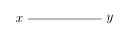
A scalar propagator joining the spacetime points x and y
Propagator Diagram

This is the most trivial example, only inserting the fields in the correlation function, and contracting them. In other words, it represents

0T[ϕ(x)ϕ(y)]0=DF(xy)\bra{0}T\left[\phi(x)\phi(y)\right]\ket{0}=D_F(x-y)

But this is too simple. Let's consider some terms that is included in the first-order λ\lambda expansion

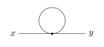
A two-point correlation diagram with a loop attached to the central interaction vertex
Two Point Correlation with 1-Loop

This diagram collectively represents ϕ(x)ϕ(y)ϕ(z)ϕ(z)ϕ(z)ϕ(z)\rule{0pt}{1.6em}\htmlData{wickopen=l2-w0-p0}{\htmlData{wickbaseline=l2-w0-p0}{\rule{0pt}{0.001em}}\phi(x)}\htmlData{wickopen=l1-w0-p1}{\htmlData{wickbaseline=l1-w0-p1}{\rule{0pt}{0.001em}}\phi(y)}\htmlData{wickclose=l2-w0-p0}{\htmlData{wickbaseline=l2-w0-p0}{\rule{0pt}{0.001em}}\phi(z)}\htmlData{wickclose=l1-w0-p1}{\htmlData{wickbaseline=l1-w0-p1}{\rule{0pt}{0.001em}}\phi(z)}\htmlData{wickopen=l1-w0-p2}{\htmlData{wickbaseline=l1-w0-p2}{\rule{0pt}{0.001em}}\phi(z)}\htmlData{wickclose=l1-w0-p2}{\htmlData{wickbaseline=l1-w0-p2}{\rule{0pt}{0.001em}}\phi(z)}, ϕ(x)ϕ(y)ϕ(z)ϕ(z)ϕ(z)ϕ(z)\rule{0pt}{1.6em}\htmlData{wickopen=l2-w0-p0}{\htmlData{wickbaseline=l2-w0-p0}{\rule{0pt}{0.001em}}\phi(x)}\htmlData{wickopen=l1-w0-p1}{\htmlData{wickbaseline=l1-w0-p1}{\rule{0pt}{0.001em}}\phi(y)}\htmlData{wickclose=l2-w0-p0}{\htmlData{wickbaseline=l2-w0-p0}{\rule{0pt}{0.001em}}\phi(z)}\htmlData{wickopen=l2-w0-p2}{\htmlData{wickbaseline=l2-w0-p2}{\rule{0pt}{0.001em}}\phi(z)}\htmlData{wickclose=l1-w0-p1}{\htmlData{wickbaseline=l1-w0-p1}{\rule{0pt}{0.001em}}\phi(z)}\htmlData{wickclose=l2-w0-p2}{\htmlData{wickbaseline=l2-w0-p2}{\rule{0pt}{0.001em}}\phi(z)}, ϕ(x)ϕ(y)ϕ(z)ϕ(z)ϕ(z)ϕ(z)\rule{0pt}{1.6em}\htmlData{wickopen=l1-w0-p0}{\htmlData{wickbaseline=l1-w0-p0}{\rule{0pt}{0.001em}}\phi(x)}\htmlData{wickopen=l2-w0-p1}{\htmlData{wickbaseline=l2-w0-p1}{\rule{0pt}{0.001em}}\phi(y)}\htmlData{wickclose=l1-w0-p0}{\htmlData{wickbaseline=l1-w0-p0}{\rule{0pt}{0.001em}}\phi(z)}\htmlData{wickopen=l1-w0-p2}{\htmlData{wickbaseline=l1-w0-p2}{\rule{0pt}{0.001em}}\phi(z)}\htmlData{wickclose=l1-w0-p2}{\htmlData{wickbaseline=l1-w0-p2}{\rule{0pt}{0.001em}}\phi(z)}\htmlData{wickclose=l2-w0-p1}{\htmlData{wickbaseline=l2-w0-p1}{\rule{0pt}{0.001em}}\phi(z)}, ϕ(x)ϕ(y)ϕ(z)ϕ(z)ϕ(z)ϕ(z)\rule{0pt}{1.6em}\htmlData{wickopen=l2-w0-p0}{\htmlData{wickbaseline=l2-w0-p0}{\rule{0pt}{0.001em}}\phi(x)}\htmlData{wickopen=l1-w0-p1}{\htmlData{wickbaseline=l1-w0-p1}{\rule{0pt}{0.001em}}\phi(y)}\htmlData{wickclose=l1-w0-p1}{\htmlData{wickbaseline=l1-w0-p1}{\rule{0pt}{0.001em}}\phi(z)}\htmlData{wickclose=l2-w0-p0}{\htmlData{wickbaseline=l2-w0-p0}{\rule{0pt}{0.001em}}\phi(z)}\htmlData{wickopen=l1-w0-p2}{\htmlData{wickbaseline=l1-w0-p2}{\rule{0pt}{0.001em}}\phi(z)}\htmlData{wickclose=l1-w0-p2}{\htmlData{wickbaseline=l1-w0-p2}{\rule{0pt}{0.001em}}\phi(z)}, ϕ(x)ϕ(y)ϕ(z)ϕ(z)ϕ(z)ϕ(z)\rule{0pt}{1.9em}\htmlData{wickopen=l3-w0-p0}{\htmlData{wickbaseline=l3-w0-p0}{\rule{0pt}{0.001em}}\phi(x)}\htmlData{wickopen=l1-w0-p1}{\htmlData{wickbaseline=l1-w0-p1}{\rule{0pt}{0.001em}}\phi(y)}\htmlData{wickopen=l2-w0-p2}{\htmlData{wickbaseline=l2-w0-p2}{\rule{0pt}{0.001em}}\phi(z)}\htmlData{wickclose=l3-w0-p0}{\htmlData{wickbaseline=l3-w0-p0}{\rule{0pt}{0.001em}}\phi(z)}\htmlData{wickclose=l1-w0-p1}{\htmlData{wickbaseline=l1-w0-p1}{\rule{0pt}{0.001em}}\phi(z)}\htmlData{wickclose=l2-w0-p2}{\htmlData{wickbaseline=l2-w0-p2}{\rule{0pt}{0.001em}}\phi(z)}, etc., in total 1212 terms, because one chooses ϕ(x)\phi(x) to contract with one of the four ϕ(z)\phi(z), and then chooses ϕ(y)\phi(y) to contract with one of the three ϕ(z)\phi(z) left, and the other two ϕ(z)\phi(z) must contract with each other. All of them evaluate to the same value DF(xz)DF(yz)DF(0)D_F(x-z)D_F(y-z)D_F(0). As you can see, with the Wick diagram, we will never need to explicitly write down all the 1212 contractions, yet still aware of what we are doing. You might feel some burden because of the DF(0)D_F(0), which should evaluate to D(0)D(0), which is divergent. Sadly, at this point we can do nothing about it, and such divergences caused by loops are to be removed systematically by renormalization. If you investigate a little bit, you will notice that all two-point Wick diagrams for ϕ4\phi^4 theory beyond λ0\lambda^0 order (i.e., the figure below, the free propagator) necessarily contain at least one loop, so unfortunately we cannot evaluate them yet. However, there exists tree-level diagrams (i.e. without loop) for the four-point correlation function, so you can try it out.

Although we lack enough power to fight all of the loops, we can get rid of a special class of them. You might have noticed that there exists diagrams (even in the first order) such as

A disconnected first-order vacuum bubble with two loops
First Order Bubble

These diagrams are characterized by the lacking of any external fields. Therefore, we can freely append any numbers of such diagrams to an existing nn-pt diagram, and form a different nn-pt diagram. Well, but isn't that stupid, because appending an disjoint diagram merely results in multiplying the corresponding contribution, and thus we can factor out those bubbles out of more meaningful nn-pt diagrams? In other words, they merely provides an equal overall factor to all diagrams without bubbles. Actually, we have already taken account for that factor. Remember the ugly vacuum normalization factor? They appear as denominators in our definition of nn-pt correlators. Of course, the vacuum normalization can be regarded as the 00-pt correlator, and it, of course, contains only bubbles, and all of them, because it can be thought of as costructed by appending bubbles to nothing, in the same manner as to other nn-pt diagrams. Therefore, we only need to evaluate those diagrams without bubbles, because of the normalization. Intuitively, the bubble diagrams represents how the free vacuum is lifted to the physical vacuum, and therefore should not enter the result because we are entirely working with physical vacuum now.

Footnotes

  1. If you are confused, think about adding extra terms to the quantum hamonic oscillator.

  2. Subtlety already arises here, because switching the vacuum somehow destroys the interpretation of particle numbers and the action of creation annihilation operators. For example: is the vacuum really free of particles? But this does not matter because we are not dealing with scattering in this section. We can only address this fact when we think about renormalization.