Free Quantum Scalar Field

Klein-Gordon Revisited

We explored around and guessed (or forced you to believe) some results about the quantized Klein-Gordon field. In this subsection, let's put those conclusions on a more solid basis. Our starting point is the Lagrangian density

$$\mathcal{S}=\int dt L=\int d^4x\,\mathcal{L}=\int d^4x\,\frac12\left(\partial^\mu\phi\partial_\mu\phi-m^2\phi^2\right)$$

We want to apply the canonical quantization process, so let's derive the Hamiltonian.

$$\pi=\frac{\partial\mathcal{L}}{\partial\dot\phi}=\dot\phi$$ $$\mathbf{H}=\int d^3\mathbf{x}\,\mathcal{H}=\int d^3\mathbf{x}\,\left(\pi\dot\phi-\mathcal{L}\right)=\frac12\int d^3\mathbf{x}\,\left(\pi^2+(\nabla\phi)^2+m^2\phi^2\right)$$

Now we impose the equal-time canonical commutation relation

$$\begin{cases} \comm{\phi(\mathbf{x})}{\pi(\mathbf{y})}=i\delta^{(3)}(\mathbf{x}-\mathbf{y})\\ \comm{\phi(\mathbf{x})}{\phi(\mathbf{y})}=0\\ \comm{\pi(\mathbf{x})}{\pi(\mathbf{y})}=0 \end{cases}$$

This should finish the quantization. However, we expect everything to look nicer with creation-annihilation operators, so we proceed.

$$\begin{cases} \phi(\mathbf{x})=\int\frac{d^3\mathbf{p}}{(2\pi)^3\sqrt{2E_\mathbf{p}}}\left(a_\mathbf{p}e^{i\mathbf{p}\cdot\mathbf{x}}+a^\dagger_\mathbf{p}e^{-i\mathbf{p}\cdot\mathbf{x}}\right)\\ \pi(\mathbf{x})=i\int \frac{d^3\mathbf{p}}{(2\pi)^3}\sqrt{\frac{E_\mathbf{p}}{2}}\left(-a_\mathbf{p}e^{i\mathbf{p}\cdot\mathbf{x}}+a^\dagger_\mathbf{p}e^{-i\mathbf{p}\cdot\mathbf{x}}\right) \end{cases}\implies \begin{cases} a_\mathbf{p}=\frac12\int d^3\mathbf{x}\,e^{-i\mathbf{p}\cdot\mathbf{x}}\left(\sqrt{2E_\mathbf{p}}\phi(\mathbf{x})+i\sqrt{\frac{2}{E_\mathbf{p}}}\pi(\mathbf{x})\right)\\ a^\dagger_\mathbf{p}=\frac12\int d^3\mathbf{x}\,e^{i\mathbf{p}\cdot\mathbf{x}}\left(\sqrt{2E_\mathbf{p}}\phi(\mathbf{x})-i\sqrt{\frac{2}{E_\mathbf{p}}}\pi(\mathbf{x})\right) \end{cases}$$

$\frac{d^3\mathbf{p}}{\sqrt{2E_\mathbf{p}}}$ is related to the orthochronous Lorentz invariant measure $d^4p\,\delta(p^2-m^2)\theta(p^0)=\frac{d^3\mathbf p}{2E_\mathbf p}$

Using the inverted equation on the right side, we can work out the commutation relation for the creation-annihilation operators.

$$\begin{aligned} \comm{\annhil{a}{p}}{\crea{a}{p^\prime}}&=\frac12\int d^3\mathbf{x}\,d^3\mathbf{y}\,e^{-i\mathbf{p}\cdot\mathbf{x}+i\mathbf{p^\prime}\cdot\mathbf{y}}\\ &\hspace{-0.5cm}\left(\sqrt{E_\mathbf{p}E_\mathbf{p^\prime}}\comm{\phi(\mathbf{x})}{\phi(\mathbf{y})}+i\sqrt{\frac{E_\mathbf{p^\prime}}{E_\mathbf{p}}}\comm{\pi(\mathbf{x})}{\phi(\mathbf{y})}-i\sqrt{\frac{E_\mathbf{p}}{E_\mathbf{p^\prime}}}\comm{\phi(\mathbf{x})}{\pi(\mathbf{y})}+\frac{1}{\sqrt{E_\mathbf{p}E_\mathbf{p^\prime}}}\comm{\pi(\mathbf{x})}{\pi(\mathbf{y})}\right)\\ &=\frac12\int d^3\mathbf{x}\,d^3\mathbf{y}\,e^{-i\mathbf{p}\cdot\mathbf{x}+i\mathbf{p^\prime}\cdot\mathbf{y}}\left(\sqrt{\frac{E_\mathbf{p^\prime}}{E_\mathbf{p}}}\delta^{(3)}(\mathbf{y}-\mathbf{x})+\sqrt{\frac{E_\mathbf{p}}{E_\mathbf{p^\prime}}}\delta^{(3)}(\mathbf{x}-\mathbf{y})\right)\\ &=\frac12\int d^3\mathbf{x}\,e^{-i\mathbf{x}\cdot(\mathbf{p}-\mathbf{p^\prime})}\left(\sqrt{\frac{E_\mathbf{p^\prime}}{E_\mathbf{p}}}+\sqrt{\frac{E_\mathbf{p}}{E_\mathbf{p^\prime}}}\right)\\ &=(2\pi)^3\delta^{(3)}(\mathbf{p}-\mathbf{p^\prime}) \end{aligned}$$

The other two pairs are trivial.

The result is quite expected. However, you may be curious about the mode expansion of the field operator, which involves both creation and annihilation operators. This is, of course, natural from the point of view of the hermicity of the field operator. But the role of the annihilation operator is indeed mysterious for now, and things get clearer once we proceed to complex scalars and think carefully about antiparticles.

With those expansions in hand, we can now express the Hamiltonian in terms of the creation-annihilation operators (Do it yourself!).

$$\mathbf{H}=\int \frac{d^3\mathbf{p}}{(2\pi)^3}\,E_\mathbf{p}\crea{a}{p}\annhil{a}{p}+\frac12\delta^{(3)}(\mathbf{0})$$

However, there is a curious term proportional to $\delta^{(3)}(\mathbf{0})$, which corresponds to the energy of the ground state of the degrees of freedom and, therefore, is proportional to the volume of the system. It is infinite due to the infinite-resolution graining of the field, but we can freely throw it away. It will not contribute to the actual energy difference that we measure. Nevertheless, it provides us with a good chance to introduce the normal ordering.

Normal Ordering

When quantizing a classical system through canonical quantization, there is an inherent ambiguity. The core of this ambiguity is that the $q$-numbers no longer commute as their $c$-number correspondents do. Similar ambiguity happens in QFT as well. In particular, when you rewrite a classical operator in terms of the creation-annihilation operators, there are many equal possibilities related by the commutation relation of the creation-annihilation operators. The problem is, such processes always produce $\delta$-functions, which lead to infinities. We would like to have an ordering of the creation-annihilation operators so that we are free of infinities. And, since we will be working intensively with the creation-annihilation operators and the vacuum state $\ket{0}$, the natural choice is to put the annihilation operators to the right, so they will touch the vacuum state. Upon imposing that, any operators that contain the annihilation operator will eliminate the vacuum state, which is also what one would do when calculating with the creation-annihilation operators.

Since such operations are very handy and we need them so often, we shall develop a notation

$$\nomo{\crea{a}{p^\prime}\annhil{a}{p^{\prime\prime}}\crea{a}{p}}=\nomo{\annhil{a}{p^{\prime\prime}}\crea{a}{p^\prime}\crea{a}{p}}=\cdots=\crea{a}{p^\prime}\crea{a}{p}\annhil{a}{p^{\prime\prime}}$$

An operator surrounded by colons $\nomo{\mathcal{O}}$ is normal-ordered, meaning that we ignore whatever order we write the creation-annihilation operators in between them; the operator is thought of as if all the annihilation operators are to the right of the creation operators.

Nobody knows why this just works in practice, but since it allows us to give all the experimentally verified results, we accept it.

Multiparticle State and Identicality

We argue in the Introduction that quantizing the field naturally gives indistinguishable particles. Let's quickly check this fact for the quantized Klein-Gordon field.

By our interpretation of the quantized field, a multi-particle state is generated by

$$\ket{\mathbf{p}_1,\mathbf{p}_2,\cdots,\mathbf{p}_n}\propto \crea{a}{\mathbf{p}_1}\crea{a}{\mathbf{p}_2}\cdots\crea{a}{\mathbf{p}_n}\ket{0}$$

Note that the creation operators are always commuting, so the sequence of how they act on the vacuum state doesn't matter. This clearly indicates that we are creating a bosonic state. In other word, the quantized Klein-Gordon field describes some type of bosonic particle.

Actually, the result goes a bit further. When we later systematically investigate the type of fields allowed in QFT, we will find that fields are essentially classified by mass and their spins. And there is a beautiful Spin-Statistics Theorem by Dirac, telling us that all particles with integer spins are bosonic, while all those with half-integer spins are fermionic. However, a detailed discussion of the topic is a bit too early for us.

Non-Equal Time and Propagators

So far, we have quantized the Klein-Gordon field and obtained a nice-looking framework to work with it. Of course, from now on, we can compute whatever we want for the theory. One of the most important quantities in QFT is the $n$-point correlation functions, which are the vacuum expectation values of $n$ products of $\phi$ at different points. Why we call it correlation functions is mysterious for now, and will be clear when we introduce Feynman's path integral later. But before we proceed to the correlators, let us compute the field operators at an arbitrary time. Be careful! Upon canonical quantization, all relations and operators have an equal reference time $t_0$.

With that being said, we push the operator to an arbitrary time $t$ using the time translation operator $e^{-i\mathbf{H}(t-t_0)}$

$$\phi(x)\equiv\phi(t,\mathbf{x})=e^{i\mathbf{H}(t-t_0)}\phi(t_0,\mathbf{x})e^{-i\mathbf{H}(t-t_0)}=\int\frac{d^3\mathbf{p}}{(2\pi)^3\sqrt{2E_\mathbf{p}}}\left(a_\mathbf{p}e^{-ip\cdot x}+a^\dagger_\mathbf{p}e^{ip\cdot x}\right)$$

Where $p^0$ in the four-momentum is identified with $E_\mathbf{p}$.

Let me explain how we get this. The core is to calculate $e^{i\mathbf{H}(t-t_0)}\crea{a}{p}e^{-i\mathbf{H}(t-t_0)}$

$$\comm{\mathbf{H}}{\crea ap}=\int \frac{d^3\mathbf{p^\prime}}{(2\pi)^3}E_\mathbf{p^\prime}\comm{\crea a{p^\prime}\annhil a{p^\prime}}{\crea ap}=\int \frac{d^3\mathbf{p^\prime}}{(2\pi)^3}E_\mathbf{p^\prime}\crea a{p^\prime}\comm{\annhil a{p^\prime}}{\crea ap}=E_\mathbf{p}\crea ap$$ $$\begin{aligned} \comm{\mathbf{H}^n}{\crea ap}&=\comm{\mathbf{H}}{\crea ap}\mathbf{H}^{n-1}+\mathbf{H}\comm{\mathbf{H}^{n-1}}{\crea ap}\\ &=E_\mathbf{p}\crea ap\mathbf{H}^{n-1}+\mathbf{H}\comm{\mathbf{H}^{n-1}}{\crea ap}\\ &=E_\mathbf{p}\crea ap\mathbf{H}^{n-1}+\mathbf{H}\left[\crea ap(\mathbf{H}+E_\mathbf{p})^{n-1}-\crea ap\mathbf H^{n-1}\right]\\ &=E_\mathbf{p}\crea ap\mathbf{H}^{n-1}+\mathbf{H}\crea ap(\mathbf{H}+E_\mathbf{p})^{n-1}-\mathbf{H}\crea ap\mathbf H^{n-1}\\ &=E_\mathbf{p}\crea ap\mathbf{H}^{n-1}+\mathbf{H}\crea ap(\mathbf{H}+E_\mathbf{p})^{n-1}-\crea ap\mathbf H^n-E_\mathbf{p}\crea ap\mathbf{H}^{n-1}\\ &=\mathbf{H}\crea ap(\mathbf{H}+E_\mathbf{p})^{n-1}-\crea ap\mathbf{H}^{n-1}\\ &=\crea ap\mathbf{H}(\mathbf{H}+E_\mathbf{p})^{n-1}+\crea apE_\mathbf{p}(\mathbf{H}+E_\mathbf{p})^{n-1}-\crea ap\mathbf{H}^{n-1}\\ &=\crea ap(\mathbf{H}+E_\mathbf{p})^n-\crea ap\mathbf{H}^n \end{aligned}$$

In those lines we used $\comm{\crea ap}{\mathbf{H}^{n-1}}=\crea ap(\mathbf{H}+E_\mathbf{p})^{n-1}-\crea ap\mathbf{H}^{n-1}$ so as to inductively prove this identity for arbitrary $n$. Note that the essence of this commutation relation is to tell that $\mathbf{H}^n\crea ap=\crea ap(\mathbf{H}+E_\mathbf p)^n$. Then, $e^{i\mathbf{H}(t-t_0)}\crea{a}{p}e^{-i\mathbf{H}(t-t_0)}=\crea ape^{i(\mathbf{H}+E_\mathbf p)(t-t_0)}e^{-i\mathbf{H}(t-t_0)}=\crea ape^{iE_\mathbf p(t-t_0)}$. Similarly for $\annhil ap$, we have $\mathbf{H}^n\annhil ap=\annhil ap(\mathbf{H}-E_\mathbf p)^n$. It is trivial to obtain the referenced equation with these identities in hand.

Good, now we have the field operator for any time and at any point. Why don't we check their commutator, so we can verify the claimed fact that QFT is causal? Let's do it.

$$\begin{aligned} \comm{\phi(x)}{\phi(y)}&=\frac{1}{(2\pi)^6}\comm{\int\frac{d^3\mathbf{p}}{\sqrt{2E_\mathbf{p}}}\left(a_\mathbf{p}e^{-ip\cdot x}+a^\dagger_\mathbf{p}e^{ip\cdot x}\right)}{\int\frac{d^3\mathbf{p^\prime}}{\sqrt{2E_\mathbf{p^\prime}}}\left(a_\mathbf{p^\prime}e^{-ip^\prime\cdot y}+a^\dagger_\mathbf{p^\prime}e^{ip^\prime\cdot y}\right)}\\ &=\frac1{(2\pi)^6}\iint\frac{d^3\mathbf{p}}{\sqrt{2E_\mathbf{p}}}\frac{d^3\mathbf{p^\prime}}{\sqrt{2E_\mathbf{p^\prime}}}\left\{e^{-ip\cdot x+ip^\prime\cdot y}\comm{\annhil ap}{\crea{a}{p^\prime}}+e^{ip\cdot x-ip^\prime\cdot y}\comm{\crea a p}{\annhil a{p^\prime}}\right\}\\ &=\int\frac{d^3\mathbf{p}}{(2\pi)^32E_\mathbf{p}}\left[e^{-ip\cdot(x-y)}-e^{-ip\cdot(y-x)}\right]\\ &=\int \frac{d^4p}{(2\pi)^3}\,\delta(p^2-m^2)\theta(p^0)\left[e^{-ip\cdot(x-y)}-e^{-ip\cdot(y-x)}\right] \end{aligned}$$

We converted back to the manifestly Lorentz invariant on-shell measure for convenience. The point is to realize that we are integrating over the orbit of the proper, orthochronous Lorentz subgroup acting on a timelike(or lightlike, but we shall assume $m>0$ for simplicity) vector $p$. Schematically, this is represented as $\sum_\Lambda f(\left<\Lambda p, x-y\right>)$, where $p$ is some representative of the orbit, say $p=(m,0,0,0)$. Since $\Lambda$ are elements of the isometry group, $\sum_\Lambda f(\left<\Lambda p, x-y\right>)=\sum_\Lambda f(\left<p, \Lambda^{-1}(x-y)\right>)=\sum_\Lambda f(\left<p,\Lambda(x-y)\right>)$.

This argument hints at how this commutator simplifies when $x-y$ is spacelike. When that is the case, there always exists an element $\Lambda$ in the proper, orthochronous Lorentz subgroup so that $y-x=\Lambda(x-y)$. Therefore, the subtraction in the referenced equation will cancel out pairwise, and thus the commutator is $0$. When $x-y$ is timelike, such an element fails to exist, and the commutator is generally non-zero. When $x-y$ is light-like, the result depends on whether $m>0$, and additional discussion is needed.¹

The calculation guaranteed us that the basic causality is preserved in QFT: when conducting measurements on spacelike-separated points $x$ and $y$, the measurements will never interfere with each other (i.e., can be measured 鈥渟imultaneously").

As we notice, the commutator of the field operator is a $c$-number. In fact, we will discuss this quantity a lot in the following sections, which is worth further discussion. To begin with, we rewrite the referenced equation in another form.

$$\begin{aligned} \comm{\phi(x)}{\phi(y)}&=\int\frac{d^3\mathbf{p}}{(2\pi)^32E_\mathbf{p}}\left[e^{-ip\cdot(x-y)}-e^{-ip\cdot(y-x)}\right]\\ &=D(x-y)-D(y-x)\\ &\sim\int \frac{d^4p}{(2\pi)^4}\frac{ie^{-ip\cdot(x-y)}}{p^2-m^2} \end{aligned}$$

In the above, we defined the function $D(x-y)=\int \frac{d^3\mathbf p}{(2\pi)^3 2E_\mathbf p}e^{-ip\cdot(x-y)}$, and we wrote a four-integral following $\sim$, because $D(x-y)$ and $-D(y-x)$ are essentially the residues of the integrand with respect to $p^0$.

The integral does not come from nowhere, and it is crucial to understand its spirit to convince yourself of the name 鈥減ropagator". The commutator of the field operator kind of measures how the measurement at $x$ affects the measurement at $y$. Physically, when such a measurement takes place, the 鈥渇ield value" at $x$ is suddenly fixed to a classical value $\phi(x)$. The consequence of the altered field state has to somehow propagate to $y$ at a finite speed due to our relativistic settings. In this way, although far from being rigorous, we are encouraged to think about how the Klein-Gordon field reacts to a disturbance. Classically, such a response is encoded in the sourced Klein-Gordon equation

$$(\square^2+m^2)\phi=\rho(x)$$

But the linearity of the Klein-Gordon equation guarantees that it suffices to work with the $\delta$-response or the kernel of the Klein-Gordon equation, which is

$$(\square^2+m^2)G(x-y)=-i\delta^{(4)}(x-y)$$

The solutions, subject to different boundary conditions, are called the Green function. And, as we shall soon find out, the propagators are just synonyms of the Green functions.

But before we can say anything, it is important to solve it first. We work with the general methodology, which we first assume is a Fourier expanded ansatz, only depending on $x-y$ due to the translational invariance and isotropicity of the equation.

$$G(x-y)=\int\frac{d^4 p}{(2\pi)^4}\tilde{G}(p)e^{-ip\cdot(x-y)}$$

With the ansatz, the equation reduces to

$$\int\frac{d^4 p}{(2\pi)^4}\tilde{G}(p)(-p^2+m^2)e^{-ip\cdot(x-y)}=-i\delta^{(4)}(x-y)$$

Finally, the equation is solved by

$$\tilde{G}(p)=\frac{i}{p^2-m^2}$$

Looks familiar? That's right, it exactly reproduces the four-integral appearing in the commutator. Our instincts are working, and the commutator is indeed somehow related to the response to a point disturbance, although we are using an unusual convention of a factor of $-i$. The appearance of $-i$, the names 鈥減ropagator", 鈥渃orrelator" and 鈥淕reen functions" will have more natural explains when we later introduce Feynman's path integral, rather than these mumbo-jumbos.

However, we are still left with one question: what is the boundary condition? Indeed, the Green function we worked out seemingly solves the equation, but we know that such a PDE is only completely solved when a proper boundary condition is specified, and there are seemingly no free parameters left for us to choose. So how do we specify the boundary condition? The answer hides in the analytic structure of the propagator.

Think carefully about the integral $\int \frac{d^4p}{(2\pi)^4}\frac{ie^{-ip\cdot(x-y)}}{p^2-m^2}$. Conventionally, the $p^0$ integral is carried out in the interval $(-\infty,+\infty)$, which seems a natural choice because $p^0$ is commonly understood as energy. But notice here that $p^0$ is not required to be on-shell, and it can even be negative (the integral is sharply peaked at the on-shell $p^0$, though). In this sense, there is no reason to require $p^0$ to be real at all. And also, when integrating over $(-\infty,+\infty)$, the path directly passes the two poles of the integrand. However, in our context, we are not obliged to consider the principal value of this integral. Instead, we can evaluate this integral along whatever path extending $(-\infty,+\infty)$, and the result still solves the equation. Since the integrand is meromorphic with two simple poles at $p^0=\pm E_\mathbf{p}$, the results of such integrals are the same if we can continuously morph between the paths without passing the poles (i.e., the paths are homotopic). Then, all possible results of this integral is classified by how the paths twist around each of the two poles.

This means that all the paths belonging to the same homotopy class describe the Green function subject to the same boundary condition, and different pole prescriptions provide different boundary conditions. Although it is hard to say whether this accounts for all possible boundary conditions, this covers all cases that we would use.

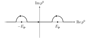
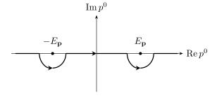
For example, if we choose a path that picks up the two poles from above (see the figure below), or equivalently, a path slightly shifted to the positive imaginary axis, the resulting Green function is called the retarded propagator. The retarded propagator get its name because it is $0$ when $x^0<y^0$, so it is the causal response to a point disturbance. Similarly, if one chooses to pick the two poles from below (the figure below), it is $0$ when $x^0>y^0$ and it is the advanced propagator.

Contour for Retarded Propagator

Contour for Advanced Propagator

Contour for Feynman Propagator

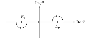
A particularly useful propagator in QFT is the Feynman propagator. It is described by the pole prescription of picking the $-E_\mathbf{p}$ pole from below and the $E_\mathbf{p}$ pole from above (the figure below). This results in

$$D_F(x-y)=\begin{cases} D(x-y) & x^0>y^0\\ D(y-x) & x^0<y^0 \end{cases}$$

A more common way to write the Feynman propagator is the $i\epsilon$-prescription, so that the poles are slightly shifted upward and downward from the axis, so the correct poles are naturally picked up.

$$D_F(x-y)=\int \frac{d^4p}{(2\pi)^4}\frac{ie^{-ip\cdot(x-y)}}{p^2-m^2+i\epsilon}\quad\epsilon>0$$

Finally, an interesting fact to mention is that all sorts of propagators (i.e., Green functions) are also described by the vacuum expectation value of the different products of two field operators, which are what two-point correlation functions really refer to. For example, the retarded propagator is often written as

$$D_R(x-y)=\theta(x^0-y^0)\bra{0}\comm{\phi(x)}{\phi(y)}\ket{0}$$

Importantly, the Feynman propagator is written as

$$D_F(x-y)=\bra{0}T\left[\phi(x)\phi(y)\right]\ket{0}$$

We introduced the time ordering in this expression. Similar to normal ordering, time ordering re-order the operators in it according to their time label, with the latest one to the leftmost. So when $x^0>y^0$, $T[\phi(x)\phi(y)]=\phi(x)\phi(y)$ and vice versa. You are recommended to check this expression yourself.

Footnotes

1. Please refer to the appendix on the Lorentz group if you find the Lorentz group particularly unfamiliar to you ↩